Jupyter Notebook
Was sind Jupyter Notebook und JupyterLab?
Jupyter (Julia, Python, R) Notebook ist die ursprüngliche Oberfläche von Project Jupyter und eine interaktive Umgebung, die es ermöglicht, Code zu schreiben und auszuführen, Daten zu visualisieren und die Arbeit an einem Ort zu dokumentieren. Es unterstützt verschiedene Programmiersprachen wie Python, R und Julia, wird aber am häufigsten mit Python verwendet. Es wird weit verbreitet in der Datenwissenschaft, im maschinellen Lernen und in der Forschung eingesetzt.
JupyterLab hingegen ist die nächste Generation der Jupyter-Oberfläche. Es baut auf der Funktionalität der Jupyter Notebooks auf und bietet eine flexiblere und leistungsfähigere Umgebung zur Arbeit mit Code und Daten.
Hier zeigen wir die Grundlagen der Arbeit mit einem Jupyter Notebook, um Text und Code zu schreiben und in verschiedenen Formaten zu speichern. Für detaillierte Informationen zu Jupyter Notebooks, siehe JupyterLabs Benutzerhandbuch.
Arbeiten mit Jupyter Notebooks
Die Verwendung von Jupyter Notebooks ist ziemlich einfach. Du kannst entweder Code oder Text, einschließlich Gleichungen, in jeder Zelle eines Notebooks schreiben und den Code interaktiv ausführen, Daten, Variablen visualisieren und analysieren und die Daten plotten. Das folgende Beispiel, einschließlich Text und Code, wurde in einem Jupyter Notebook geschrieben.
Zuerst öffnest du ein Jupyter Notebook, das automatisch in deiner Umgebung gespeichert wird. Der Standardpfad ist dein Home-Verzeichnis. Wenn du jedoch in ein Verzeichnis wechselst und dann ein Notebook öffnest, wird es im aktuellen Verzeichnis gespeichert. Du kannst dein Notebook umbenennen, indem du mit der rechten Maustaste klickst und “Umbennen” auswählst.
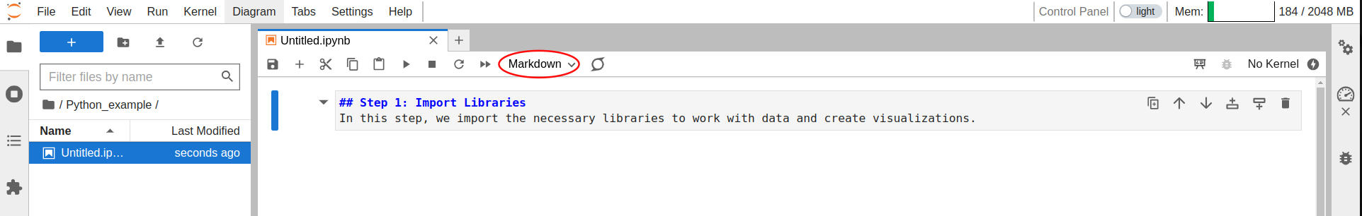
Jetzt können wir mit dem Schreiben unseres Notebooks beginnen! Wir können mit dem Schreiben eines Textes beginnen, wie den, den du in Schritt 1 im folgenden Beispiel siehst. Wenn du die Zelle in einen Text umwandeln möchtest, musst du Markdown im Dropdown-Menü des Notebooks oben (wo du Code siehst) oder mit der Tastenkombination m auswählen.
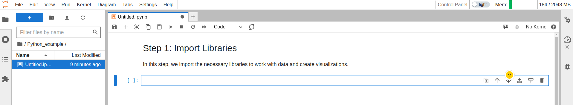
Wenn du Enter + Shift drückst, führst du die Zelle aus und jetzt siehst du, dass du einen schönen Text hast!
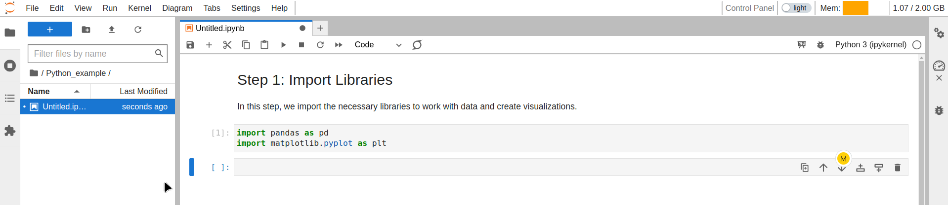
Dann kannst du in der nächsten Zelle einen Code-Ausschnitt schreiben und ihn ausführen.
Du kannst auch Zellen per Drag & Drop umordnen, Zellen löschen und leicht Zellen zu deinem Notebook hinzufügen.
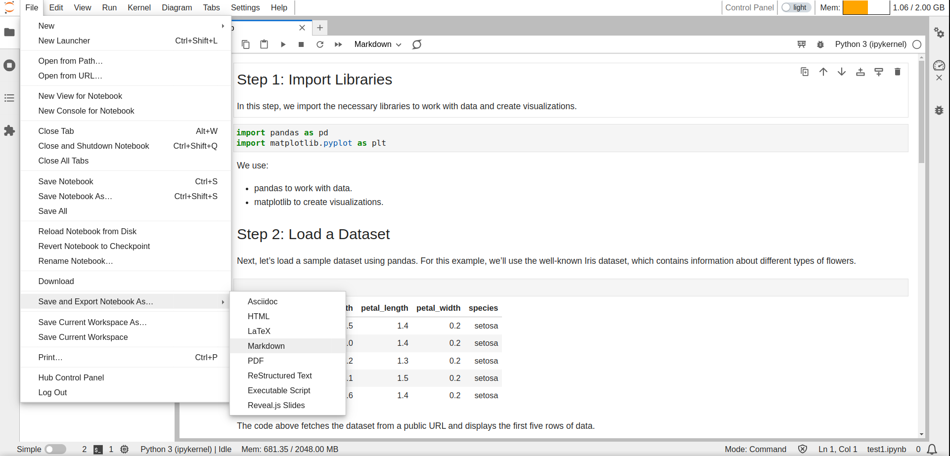
Wenn du mit deinem Notebook fertig bist, kannst du es in andere Formate exportieren, einschließlich Markdown, PDF usw. Das kannst du über Datei/Speichern und Notebook als ... exportieren.
Jupyter Notebooks werden von Kerneln angetrieben, die den von dir geschriebenen Code ausführen. Jeder Kernel verbraucht Speicher und Rechenressourcen, daher ist es wichtig, die Kerne zu verwalten. Das hilft dabei, deine Umgebung schnell und reaktionsfähig zu halten. Siehe die Seite Kerne und Terminals verwalten dieser Anleitung und JupyterLabs Benutzerhandbuch für weitere Informationen.
Zum Üben kannst du das folgende Beispiel (in Python) durcharbeiten, mit Daten arbeiten und sie in einem Jupyter Notebook analysieren.
Beispiel: Analysieren und Visualisieren von Daten in Python mit einem Jupyter Notebook
Lass uns ein einfaches Beispiel durchgehen, bei dem wir einen Datensatz laden, eine grundlegende Analyse durchführen und eine Visualisierung erstellen, alles innerhalb eines Jupyter Notebooks.
Schritt 1: Bibliotheken importieren
In diesem Schritt importieren wir die notwendigen Bibliotheken, um mit Daten zu arbeiten und Visualisierungen zu erstellen.
import pandas as pd
import matplotlib.pyplot as plt
Wir verwenden:
- pandas, um mit Daten zu arbeiten.
- matplotlib, um Visualisierungen zu erstellen.
Schritt 2: Datensatz laden
Als Nächstes laden wir einen Beispiel-Datensatz mit pandas. Für dieses Beispiel verwenden wir den bekannten Iris-Datensatz, der Informationen über verschiedene Blumenarten enthält.
# Iris-Datensatz laden
url = "https://raw.githubusercontent.com/mwaskom/seaborn-data/master/iris.csv"
data = pd.read_csv(url)
# Die ersten fünf Zeilen des Datensatzes anzeigen
data.head()
| sepal_length | sepal_width | petal_length | petal_width | species | |
|---|---|---|---|---|---|
| 0 | 5.1 | 3.5 | 1.4 | 0.2 | setosa |
| 1 | 4.9 | 3.0 | 1.4 | 0.2 | setosa |
| 2 | 4.7 | 3.2 | 1.3 | 0.2 | setosa |
| 3 | 4.6 | 3.1 | 1.5 | 0.2 | setosa |
| 4 | 5.0 | 3.6 | 1.4 | 0.2 | setosa |
Der obige Code holt den Datensatz von einer öffentlichen URL und zeigt die ersten fünf Datenzeilen an.
Schritt 3: Datenanalyse
Lass uns eine grundlegende Analyse des Datensatzes durchführen. Zum Beispiel können wir die durchschnittliche Kelchlänge für jede Blumenart berechnen.
# Durchschnittliche Kelchlänge nach Art berechnen
average_petal_length = data.groupby('species')['petal_length'].mean()
average_petal_length
species
setosa        1.462
versicolor    4.260
virginica     5.552
Name: petal_length, dtype: float64
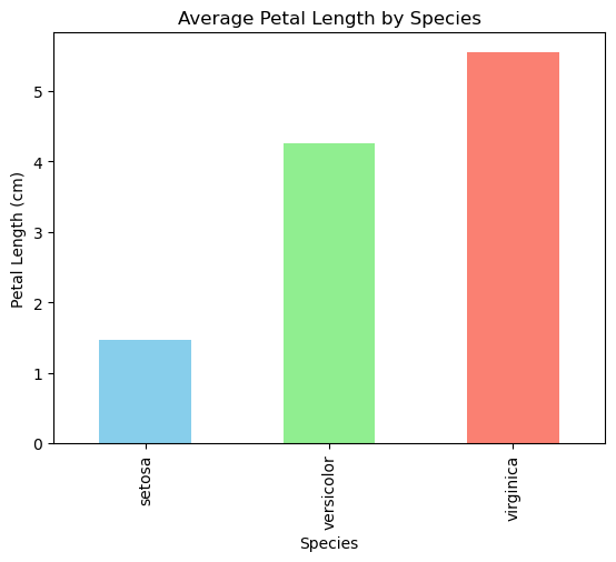
Schritt 4: Datenvisualisierung
Jetzt lassen wir uns ein einfaches Balkendiagramm erstellen, um die durchschnittliche Kelchlänge für jede Art zu visualisieren.
# Balkendiagramm für die durchschnittliche Kelchlänge nach Art erstellen
average_petal_length.plot(kind='bar', color=['skyblue', 'lightgreen', 'salmon'])
plt.title('Durchschnittliche Kelchlänge nach Art')
plt.ylabel('Kelchlänge (cm)')
plt.xlabel('Art')
plt.show()
Nützliche Links: